Appendix: Crystal Growth Theory and Computational Protocol

Crystal growth is one of those areas where theory meets practice in fascinating (and often frustrating) ways. You can have the most beautiful theoretical understanding of molecular interactions, but when it comes to predicting what shape crystals will actually grow into, you quickly realize that the devil is in the details - and there are a lot of details.

This appendix walks through the theory behind occ cg calculations, but more importantly, explains why we do things the way we do them and where the approximations might break down. If you're going to use these methods in practice, you need to understand not just how they work, but when they're likely to give you nonsense.

Crystal Growth Models: From Molecular Interactions to Morphology

The Terrace-Step-Kink Model

Terrace-step-kink model of crystal growth showing molecular attachment sites

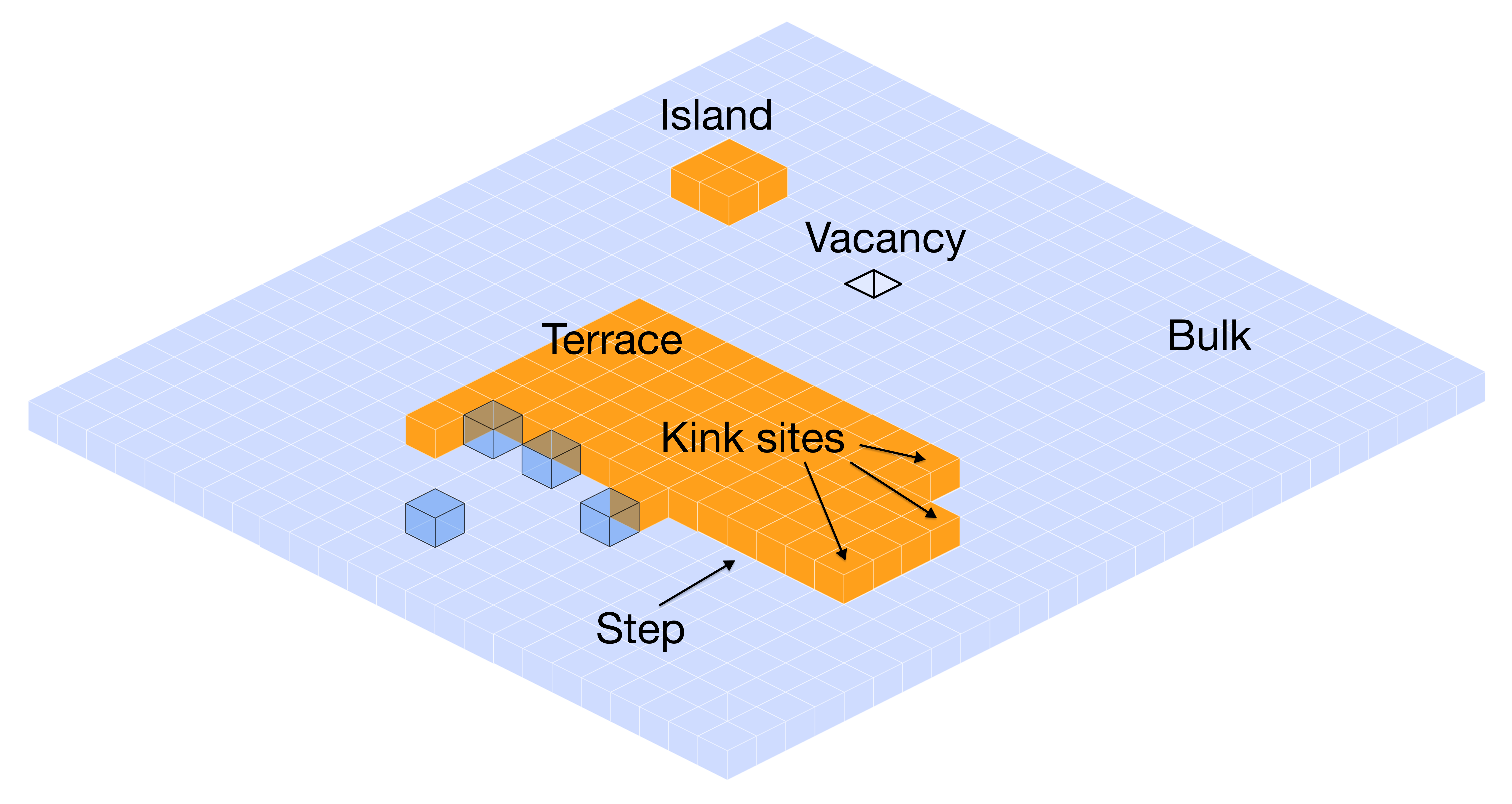
Real crystal surfaces aren't the perfect flat planes you see in textbook diagrams. They're messy, with steps, kinks, and all sorts of irregularities. The terrace-step-kink (TSK) model is our way of making sense of this mess:

• Terraces: The relatively flat bits - molecules here are well-coordinated but hard to access
• Steps: Where different terraces meet - linear defects that are somewhat exposed
• Kinks: The really interesting spots - corners along step edges where molecules can easily attach

Here's the key insight: crystals grow fastest at kink sites. Why? It's a Goldilocks situation - kink sites provide enough coordination to bind strongly, but they're still accessible enough for new molecules to actually reach them. A molecule trying to attach to the middle of a flat terrace has a much harder time because it can't make as many contacts with its neighbors.

The attachment energy tells you how much a face wants to grow:

$E_{\text{att}} = \sum_{\text{neighbors}} (E_{\text{crystal}}^{AB} - E_{\text{solvent}}^{AB})$

This is just saying: "How much more stable is this molecule when it's attached to the crystal versus when it's dissolved in solution?" If that number is large and negative (i.e., much more stable in the crystal), that face will grow fast. If it's small, the face grows slowly and ends up dominating the final crystal shape.

Slow faces dominate morphology

This is counterintuitive! The faces that grow slowly are the ones you see on the final crystal, because the fast-growing faces quickly disappear. It's like natural selection for crystal faces.

Thermodynamic vs. Kinetic Control

Here's where things get philosophically interesting. Are crystals lazy or impatient?

Thermodynamic control: The crystal is lazy - it takes its time and ends up in the most stable shape possible. Surface energies determine the final shape because everything has time to equilibrate. This gives you nice, well-formed crystals.

Kinetic control: The crystal is impatient - it grows so fast that it gets trapped in whatever shape it happens to be forming. You get weird morphologies like needles, dendrites, or those snowflake patterns that form when water freezes quickly.

The methods we're discussing here assume thermodynamic control. We're basically saying that the activation barriers for attachment and detachment are similar for all the different surface sites, so the thermodynamic driving force (the attachment energy) is a good proxy for the relative growth rates.

When kinetics matters

This assumption breaks down when:

• You're growing very fast (high supersaturation)
• Different faces have very different activation barriers
• Solvent molecules get in the way differently on different faces
• Mass transport becomes limiting

If you see weird crystal shapes that don't match your predictions, kinetics might be taking over.

Monte Carlo Crystal Growth Simulation

The CrystalGrower Approach

Monte Carlo simulation is perfect for crystal growth because, let's face it, crystal growth is fundamentally a random process. Molecules are constantly bumping around in solution, occasionally sticking to or falling off the crystal surface. We can't predict exactly when each molecule will attach, but we can predict the probabilities.

CrystalGrower treats the crystal as a 3D lattice where each site can either be occupied (molecule present) or empty. Then it plays a gigantic game of molecular roulette:

1. Pick a site: Randomly choose a surface site that could potentially change
2. Pick an event: If it's empty, try to stick a molecule there. If it's occupied, try to remove it
3. Calculate the energy: How much would this move cost or gain?
4. Roll the dice: Accept or reject based on $P = \exp(-\Delta G / k_B T)$
5. Repeat: Do this millions of times until you get bored (or the crystal reaches equilibrium)

The beauty is that this automatically gives you the right equilibrium distribution without having to solve any complicated differential equations.

Supersaturation: The Driving Force

In real experiments, you don't grow crystals from perfectly saturated solutions - that would take forever. You need supersaturation to provide the driving force. The chemical potential difference tells you how "hungry" the system is to form crystals:

$\Delta \mu = k_B T \ln(S)$

Where S is the supersaturation ratio (how much more concentrated your solution is compared to the saturation concentration). This gets added to your attachment energy:

$\Delta G_{\text{total}} = \Delta G_{\text{attachment}} - \Delta \mu$

The trick is getting the supersaturation right. Too low and nothing happens. Too high and you get kinetic effects (or worse, you crash everything out at once in an amorphous mess).

A typical simulation recipe:

• Start with ridiculously high supersaturation (S ~ 100) to get nucleation going
• Slowly dial it back to equilibrium over 100,000 steps
• Let it cook for 4-5 million total steps until the morphology stabilizes

Simulation time vs. real time

These Monte Carlo steps don't correspond to real time - they're just a way of sampling configuration space. Don't try to convert them to actual growth rates without a lot more work.

What the Simulation Needs From You

Here's the problem: the Monte Carlo simulation needs to know the energy for every possible way a molecule can attach to or detach from the crystal surface. And there are a lot of possible environments - corner sites, edge sites, different orientations, different local coordination numbers, etc.

Traditionally, people would just fit all these energies to match experimental crystal shapes. This works, but it's a nightmare of parameter optimization, and you need experimental data for every system you want to study.

The occ cg approach tries to predict these energies from first principles, which sounds great in theory but requires some clever tricks to make it work in practice.

Computational Energy Protocol: The "How" and "Why"

The Big Picture

Here's what we're trying to do: start with just a crystal structure and a solvent choice, and end up with a predicted crystal morphology. The magic happens through a computational pipeline that combines several different methods:

1. CE-1p model: Get intermolecular interactions quickly (without breaking the bank)
2. SMD solvation: Figure out how much the solvent likes each molecule
3. Energy partitioning: Break everything down into bite-sized pieces for the simulation
4. CrystalGrower: Run the actual growth simulation

Each step has its own approximations and potential failure modes, so let's dig into them.

Step 1: Get the Lattice Energies (Without Going Broke)

This is where CE-1p comes to the rescue. You need intermolecular interaction energies for all the molecular pairs in your crystal, but doing full quantum mechanical calculations for every dimer would take approximately forever.

CE-1p gives you quantum mechanical quality for the price of a force field calculation:

$U_{\text{latt}} = \frac{1}{2} \sum_{A} \sum_{r_n^{AB} < r_{\text{max}}} E^{AB}_{\text{CE-1p}}$

The factor of 1/2 is there because we're double-counting pairs (A interacting with B is the same as B interacting with A).

Why CE-1p is brilliant:

• No geometry optimization needed: Use the experimental crystal structure as-is
• ~12x speed boost: Avoid the expensive dimer SCF calculation
• One parameter to rule them all: k = 0.78 works for basically everything
• Periodic table coverage: H to Rn (yes, even radioactive stuff)

Distance matters

We use nearest atom-atom distance ($r_n^{AB}$), not center-of-mass distance. For weird-shaped molecules, the center of mass can be misleading - what matters is how close the electrons actually get to each other.

Step 2: Long-Range Interaction Assignment

Challenge: CrystalGrower focuses on nearest-neighbor interactions, but long-range contributions can be significant, especially for polar molecules.

Solution: Assign non-nearest neighbor interactions to nearest neighbors based on directional overlap:

For a non-nearest neighbor interaction AC, partition its energy among nearest neighbors AB:

$E_{LR}^{AB} = \sum_{AC \notin NN} \frac{\vec{r}^{AB} \cdot \vec{r}^{AC}}{w_{\text{tot}}^{AC}} E^{AC}$

Where the total weight is: $w_{\text{tot}}^{AC} = \sum_{AB \in NN} \vec{r}^{AB} \cdot \vec{r}^{AC}$

This preserves total energy while maintaining directional character of long-range interactions.

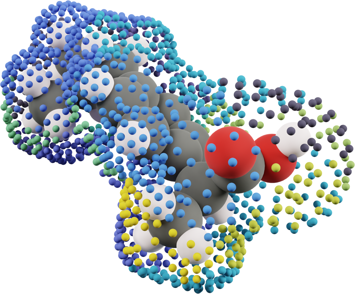
Step 3: Solvation Energy Calculation

SMD Continuum Model: Calculates solvation free energies using the Solvation Model based on Density:

$\Delta G_{\text{solv}} = \Delta G_{\text{EP}} + \Delta G_{\text{CDS}} + \Delta G_{\text{std}}$

Components:

• $\Delta G_{\text{EP}}$: Electronic polarization from self-consistent reaction field
• $\Delta G_{\text{CDS}}$: Cavitation, dispersion, and solvent structure effects
• $\Delta G_{\text{std}}$: Standard state correction (7.91 kJ/mol)

Computational procedure:

1. Gas-phase SCF calculation for isolated molecule
2. Solvated SCF calculation with continuum environment
3. Surface generation for cavitation/dispersion terms
4. Combine all contributions for total solvation free energy

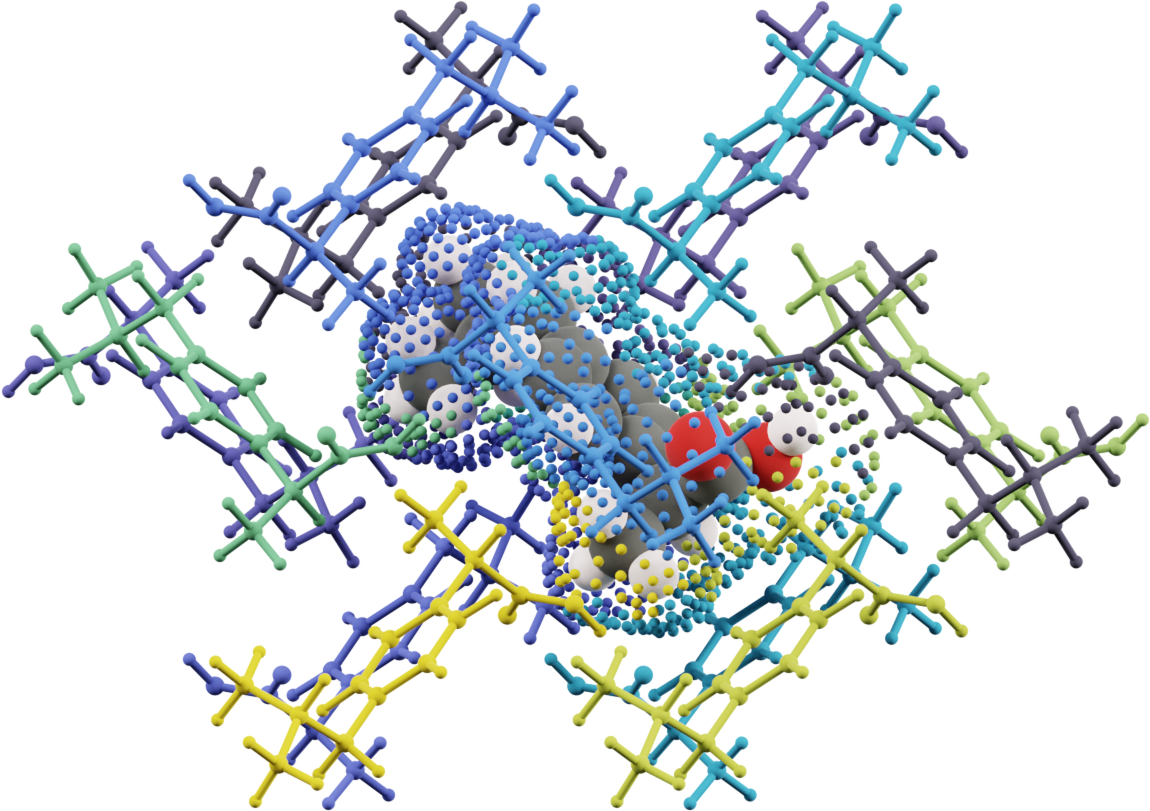
Step 4: Solvation Energy Partitioning

SMD solvation surface with partitioning for neighboring interactions

Innovation: Partition bulk solvation free energies into interaction-specific contributions based on molecular surface analysis.

Procedure:

1. Surface orientation: Rotate continuum surface to match crystal environment
2. Surface assignment: Assign each surface point to nearest neighboring molecule
3. Energy partitioning: Use surface area weights to distribute solvation energy

For asymmetric crystal-solution interfaces:

$\Delta G_{\text{solv}}^{\text{total}} = \Delta G_{\text{solv}}^{\overrightarrow{AB}} + \Delta G_{\text{solv}}^{\overrightarrow{BA}} + \frac{\Delta G_{\text{solv}}^{\overrightarrow{AB}} - \Delta G_{\text{solv}}^{\overrightarrow{BA}}}{2}$

This maintains energy conservation while preserving interface asymmetry.

Step 5: Crystal Growth Simulation

Crystal growth environment showing neighboring molecules and interaction assignment

Final step: Use computed interaction energies in CrystalGrower Monte Carlo simulation.

Total attachment energy for each surface site:

$E_{\text{attachment}} = \sum_{\text{neighbors}} (E_{\text{CE-1p}}^{AB} + E_{LR}^{AB} + \Delta G_{\text{solv}}^{AB})$

The simulation predicts:

• Surface energies: Cost of creating crystal-solution interfaces
• Growth rates: Relative rates for different crystal faces
• Morphology: Final crystal shape from competition between faces
• Solvent effects: How different solvents modify crystal shape

Physical Interpretation and Applications

Energy Landscape

Thermodynamic cycle connecting crystal lattice energy, solvation energy, and surface site energies

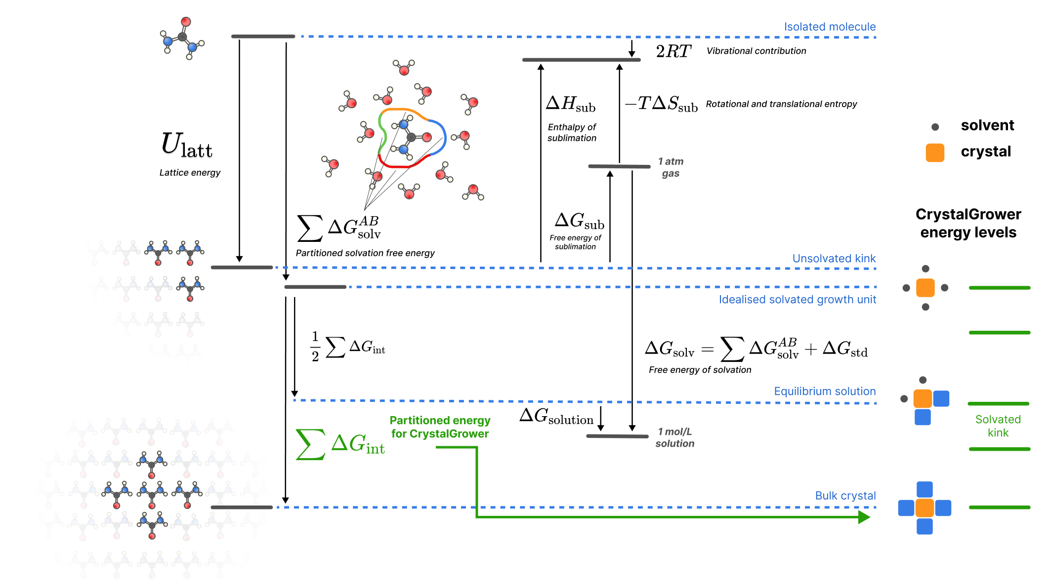
The complete thermodynamic description connects molecular interactions to macroscopic properties:

• Gas phase: Isolated molecule energy (reference state)
• Solution: Molecule stabilized by solvation energy
• Kink site: Molecule partially coordinated in crystal
• Bulk crystal: Molecule fully coordinated (maximum stability)

The energy differences between these states determine solubility, growth rates, and morphology.

Solvent Effects on Morphology

Different solvents produce different crystal shapes through modified competition:

• Polar solvents: Strongly solvate polar molecular groups, slowing growth of faces that expose these groups
• Nonpolar solvents: Weakly solvate hydrophobic regions, allowing faster growth
• Hydrogen bonding: Specific interactions can dramatically modify face-specific growth rates

Computational Advantages

Efficiency: The protocol is designed for rapid screening:

• CE-1p: ~5 seconds per dimer vs ~60 seconds for full QM
• SMD: Converged in 2 SCF calculations
• Partitioning: Fast geometric algorithm
• Total: ~1 hour for typical pharmaceutical molecule

Accuracy: Validation studies show:

• Morphology prediction: Correct major faces for organic crystals
• Solvent effects: Reproduces experimental trends
• Energies: 10-30% typical error vs experimental values

General applicability:

• No empirical fitting required
• Works for any crystal structure + solvent combination
• Handles elements H through Rn
• Suitable for high-throughput screening

Implementation: occ cg Command

Basic Usage

occ cg crystal.cif --model=ce-1p --solvent=water --radius=4.1 --surface-energies=10

Key Parameters

• --model: Energy model (ce-1p recommended for speed/accuracy balance)
• --solvent: Solvent for SMD calculations (water, ethanol, acetonitrile, etc.)
• --radius: Cutoff distance for nearest-neighbor definition (Å)
• --surface-energies: Number of crystal faces to analyze
• --max-radius: Maximum distance for long-range interactions (default 30 Å)

Output Files

The calculation produces several output files:

• Interaction energies: CE-1p energies for all molecular pairs
• Solvation energies: SMD results and surface partitioning
• Surface analysis: Face identification and attachment energies
• CrystalGrower input: Files ready for Monte Carlo simulation
• Morphology prediction: Final crystal shape visualization

Integration with CrystalGrower

The occ cg output can be directly used with CrystalGrower for detailed morphology simulation:

1. Energy calculation: occ cg computes all required interaction energies
2. File preparation: Automatic generation of CrystalGrower input files
3. Simulation: Run Monte Carlo crystal growth with predicted energies
4. Analysis: Compare predicted vs experimental morphologies

Limitations and Future Directions

Current Limitations

• Thermodynamic approximation: Assumes similar transition state barriers
• Continuum solvation: No explicit solvent molecules or specific binding
• Rigid molecules: No conformational changes upon crystallization
• Pure phases: No impurities or additives

Potential Improvements

• Explicit solvation: Include specific solvent-solute interactions
• Kinetic effects: Incorporate growth barriers and surface reconstruction
• Temperature dependence: Extend beyond standard conditions
• Multi-component systems: Handle co-crystals and solid solutions

The current methodology provides an excellent starting point for crystal engineering applications, with systematic improvements possible as computational resources and theoretical methods continue to advance.